Supplement to “Choosing a charge law for four dimensions: what 1/r does to atoms and the periodic table”
The notation and appendices of paper 1, on a page of their own. References to the main text link back to the paper.
Notation
Atomic units throughout: , and the law’s constant is 1, so two charges and a distance apart have the energy in hartree with in bohr. “Ours” is our own three-dimensional world. The subshell letters s, p, d, f (upright) are , and in four dimensions a subshell of angular momentum holds electrons. Bold letters are vectors.
| symbol | meaning | from |
|---|---|---|
| the number of dimensions of space: 3 in ours, 4 here | §2 | |
| distance from the nucleus, or between two charges | §2 | |
| , ; | points of -dimensional space; the coordinates of | §2.1 |
| the potential energy of one electron | §2.1 | |
| the strength of Gauss’s pull in four dimensions | §2.1 | |
| , | a one-electron Hamiltonian and its wavefunction | §2.1 |
| , | gradient and Laplacian in dimensions | §2.1 |
| a scale factor, | §2.1 | |
| the power of a wavefunction close to the nucleus | App. F.1 | |
| a one-electron (orbital) energy, in hartree | §3 | |
| a total energy; (bold) is the electric field | §2.1 | |
| the inner end of a calculation’s radial grid | App. F.1 | |
| , | momentum | §2.2 |
| , | Planck’s constant over and the electron’s mass (both 1 in atomic units) | §2.2 |
| the exponent of a trial law ( is the pinned law, Gauss’s) | §2.3 | |
| the nuclear charge, the element’s number | §2.3 | |
| , | angular momentum in the plane ; the Runge–Lenz vector | §2.3 |
| wavenumber (Fourier space); is the Fermi wavenumber | §2.5 | |
| , | the principal and angular quantum numbers | §2.3 |
| the radius of a spherical shell of charge | §2.4 | |
| , the ratio of the two radii | §2.4 | |
| the shell kernel: a shell’s potential over the shell theorem’s, in ours | §2.4 | |
| , | the shell kernel and the local-exchange constant under a law ; , | App. F.8 |
| the distance from an atom to an outside charge, or between two atoms | §2.4 | |
| an atom’s over its electrons; , for atoms A and B | §2.4 | |
| an atom’s dipole polarizability at imaginary frequency; the static one | App. J.1 | |
| , | the coefficients of two like atoms’ dispersion and permanent pull , | §7 |
| , the distance inside which dispersion is the larger | §7 | |
| the spread of a d subshell’s one-electron levels in a ligand field | App. H.5 | |
| an electric potential | App. F.5 | |
| , | angular frequency; the speed of light | App. F.5 |
| a density: of charge in §2.5, of electrons in an atom from §3 | §2.5 | |
| , | the vacuum’s permittivity and permeability | §2.5 |
| the lens vacuum’s length: permittivity , permeability | §2.5 | |
| the exponent of the nonlinear vacuum, | App. F.5 | |
| , , | electric field, displacement, magnetic field | §2.5 |
| a number of electrons, or of atoms | App. F.7 | |
| the radial function: with a harmonic of degree | §3 | |
| , the angular momentum the radial equation sees | §3 | |
| , , | exchange energy per electron, exchange potential, and the exchange constant: | §3 |
| the grid’s step in | App. G.5 | |
| , | an open subshell’s total spin and its projection | App. H.1 |
| the radial (Slater) integrals of the repulsion within a subshell, | §5.2 | |
| the Gegenbauer polynomial , the 3-sphere’s analogue of Legendre’s | §5.2 | |
| the angle between two electrons, seen from the nucleus | §5.2 | |
| over a term, its share of | §5.2 | |
| the polar angle on a sphere | App. A | |
| , (upright) | complete elliptic integrals of the first and second kind | App. A |
| the Legendre polynomial | App. A | |
| the volume of the unit ball in dimensions ( for ) | App. B | |
| ; | the spatial Dirac matrices of 4 + 1 dimensions; their product, time’s | App. F.6 |
| the free electron’s Dirac Hamiltonian | App. F.6 | |
| ; | a wavepacket’s width; its weight in the negative-energy states | App. F.6 |
| the repulsion between two copies of one charge density | App. F.6 |
A · The 4D kernel
A thin spherical shell of unit charge and radius , felt at radius , gives the potential , where and is the law’s averaged over the shell. On the 3-sphere the average over directions carries the weight , so
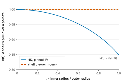
In ours the same average, with weight , is exactly 1 for every : the shell theorem. In four dimensions it isn’t. The integral has a closed form in the complete elliptic integrals and of modulus ,
which gives (since ), and the series
Each term is
times the average of the Legendre polynomial
over the 3-sphere; the odd ones vanish. The solver evaluates
by Simpson’s rule in
with 400 intervals, tabulated at 2001 points of
and interpolated. The closed form agrees with that quadrature to 2.7 ×
10⁻¹⁵ for
up to 0.9 (ledger kernelclosed); nearer 1 the quadrature’s
own error dominates, a few parts in
.
The series’ first correction is the far pull of section 7. A cloud of electrons around a nucleus , seen from a distance outside it, gives . A neutral atom therefore acts on an electron through with , and two neutral atoms on each other through (section 7). Figure A1 draws , and the potential inside and outside a shell.
B · The 4D electron gas
The solver’s exchange is the local form of the uniform electron gas of the same dimension and the same law. In dimensions a spin-unpolarized Fermi sea of density has , with the volume of the unit ball ( for ). Its kinetic energy per volume is : in ours (Thomas–Fermi’s 2.8712), in four dimensions. Its exchange energy per volume is . In ours = 0.738559, Dirac’s constant. In four dimensions under the pinned , with the Fermi sea’s density matrix built on the Bessel function and the integral , it is = 0.601802. These agree with Loos and Gill’s expressions for the -dimensional gas (2016). The selftest checks the textbook values in ours and the 4D integral (blocks 4 and 18). The potential each electron feels is , spin-polarized as in section 3 (each spin’s own density doubled), with each electron’s own share taken out.
C · Numerical convergence
The solver’s stop. The self-consistent field stops
when the total energy changes by less than 10⁻⁷ hartree between
iterations. Re-solving 19 atoms (4D 2, 4D 7, 4D 12, 4D 13, 4D 22, 4D 26,
4D 50, 4D 51, 4D 68, 4D 78, 4D 101, 4D 128, 4D 138, ours 2, ours 10,
ours 11, ours 18, ours 26, ours 36) with the stop at 10⁻¹² moves no
total energy by more than 2.7 × 10⁻⁷ hartree and no first ionization by
more than 2.8 × 10⁻⁷ (ledger converged).
The radial grid. The baked grid has 700 points from
10⁻⁵ to 150 bohr, logarithmic with step 0.02364. 11 atoms (4D 2, 4D 12,
4D 13, 4D 22, 4D 50, 4D 78, 4D 128, 4D 138, ours 10, ours 18, ours 36)
were re-solved on six other grids, each changing one parameter (ledger
grid):
| change from the baked grid | largest |ΔE| (hartree) | largest |Δ ionization| (hartree) |
|---|---|---|
| N 500 | 2.0 × 10⁻² | 1.4 × 10⁻⁴ |
| N 1000 | 1.0 × 10⁻² | 7.2 × 10⁻⁵ |
| r₀ 10⁻⁴ | 6.7 × 10⁻² | 3.8 × 10⁻⁵ |
| r₀ 10⁻⁶ | 5.4 × 10⁻³ | 4.2 × 10⁻⁵ |
| r_max 100 | 1.0 × 10⁻³ | 6.9 × 10⁻⁶ |
| r_max 250 | 1.3 × 10⁻³ | 8.9 × 10⁻⁶ |
The total energies of the heaviest atoms move by up to 6.7 × 10⁻² hartree, 2.4 × 10⁻⁵ of themselves, with the innermost point. The ionization energies, the differences the paper’s chemistry uses, move by at most 1.4 × 10⁻⁴ hartree.
D · The law calculations
Section 2’s arguments use a separate
one-electron solver (laws.js), so that the grid’s inner end
can be moved. It uses the radial equation with
on a logarithmic grid of 6000 points, counts the nodes of an outward
Numerov solution at a trial energy, and bisects on the count to
relative; a level that falls with the inner end of the grid is a fall to
the centre. Its check is 4D hydrogen, −0.22222222 hartree against
.
Gauss’s
.
At
= 0.45 there is no bound level on any grid. At
= 0.7 the lowest level is −5.87 × 10³, −5.87 × 10⁵ and −5.87 × 10⁷
hartree with the inner end at
,
and
bohr:
= −0.00587 and −0.00587, a fall to the centre set by
(ledger gauss). The boundary between the two is Hardy’s
constant
(Barbatis
2024), which with the kinetic energy
puts the critical
at
(Landau and Lifshitz 1977, sec. 35).
Power laws
.
The splitting of 2p from 2s, as a fraction of the shell’s binding, is
−6.2 % at
,
5 × 10⁻¹⁰ % at
,
+15.4 % at
and +64.0 % at
.
For 3d against 3s it is −9.2 %, +21.9 % and +78.3 % (ledger
uniqueness). Only
keeps a shell together.
E · Checks against our world
E.1 Hydrogen. One electron needs no search and no exchange, and four-dimensional hydrogen has an exact answer: hartree, so for the ground state. The solver gives −0.22222.
E.2 Two electrons.
Helium-like atoms in four dimensions are checked against an independent
code, Hartree–Fock in a Gaussian basis written for any dimension
(gauss.js), and the same atoms in ours against PySCF at the
MP2 level (selftest blocks 17 and 43). The two codes share no part of
the radial solver. From outside, the only accurate four-dimensional
numbers we have been able to read are correlated variational energies
for helium-like ions (Escobar-Ruiz et al.
2021). Hartree–Fock (hf.js, appendix G.12) lies above them by 0.012–0.014 hartree for
= 2–10. That order is expected but not compelled: two restricted
variational families need not be nested, so a correlated trial energy is
not bound to lie below Hartree–Fock’s. The gap has the size and sign of
a correlation energy, which makes it a consistency check rather than a
benchmark against a Hartree–Fock limit. A four-dimensional Hartree–Fock
limit to test against (Loeser and Herschbach 1986) is in tables
we have not obtained.
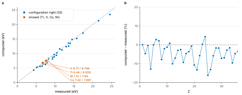
E.3 Our own table, and the solver’s lean toward d. The same solver, the same law (in ours 1/r is Gauss’s) and the same search, run in three dimensions, gives 32 of 36 of our measured ground configurations. The four it misses, titanium, vanadium, cobalt and nickel, each take one d electron too many against 4s, the known lean of local exchange toward d. The misses have one cause. Moving an electron from 4s into 3d comes out too cheap in every 3d atom we can compare (eV, the solver against measured: Sc 0.14 against 1.43, Ti −0.89 against 0.81, Fe 0.51 against 0.87, Co −0.35 against 0.42, Ni −1.16 against −0.03), short by 0.37–1.70 eV and a mean 1.05, always in d’s favour. The measured values are differences of each configuration’s lowest term, its levels averaged with weights , from NIST’s level tables (Sansonetti and Martin 2005), because the solver has no spin–orbit coupling and lands each configuration in its lowest term. Taking the lowest level of each instead moves them by at most 0.06 eV and turns nickel’s sign (+0.03 rather than −0.03). That is local exchange without correlation. Resolving every open subshell’s whole term structure doesn’t remove it. With that correction (the lowest term less the average of the maximum-spin arrangements, which is what a spherically averaged field stands for), the bias stays at 1.05 eV and the configurations get worse, 26 of 32 against 28 of 32. So the paper corrects only Hund’s first rule (section 5), the one thing a spin-polarized averaged field cannot represent. Its first ionization energies are off by a median 4.3 % and at most 16.2 % (figure A2). That is the accuracy to expect of the 4D table: a method that gets our transition metals mostly right and our ionizations to a few percent, not a spectroscopic one.
E.4 Ions. Each ion of ours searched for its own ground state, rather than made by taking one electron from the atom’s configuration, changes no first ionization. Searched the same way, our +2 and +3 ions give second and third ionization energies within a median 2.0 % and 1.4 % of measured ones (Kramida et al. 2026) (worst V, 7 % and C, 4 %), closer than the first ionizations’ 4.3 %, and they lose their 4s electrons before 3d, as measured (Fe⁺ 3d⁶4s, Fe²⁺ 3d⁶, Fe³⁺ 3d⁵). In four dimensions the 3d row’s ions do the same. Elements in the first half of the 4d and 5d blocks, and the two that open row 6’s f block with a 5d electron, instead give up a d electron at +1 or +2 while keeping the outer s (53–56, 58, 61, 81–82, 114–118, 120, 122), as our yttrium and lutetium do (Y⁺ 5s², Lu⁺ 6s²). The same search for anions gives our electron affinities where the extra electron is bound by the field and exchange: the p-block acceptors (C 1.32 against 1.262, Si 1.30 against 1.39, Ge 1.25 against 1.233, Al 0.40 against 0.433, F 2.80 against 3.401, Cl 3.15 against 3.613, O 0.71 against 1.461 eV, measured second). It also finds every anion that should be unbound to be unbound: the noble gases, beryllium, magnesium and nitrogen. It fails where correlation does the binding (H -0.33 against 0.754, Li -0.08 against 0.618, Na -0.02 against 0.548, P -0.10 against 0.746). In ours, then, the method’s affinities hold above about 0.7 eV and not below (the measured values are from Rienstra-Kiracofe et al. (2002)). That is a calibration in our world, not an error bar for four dimensions: an affinity near threshold there would need its own checks, a wider radial grid for the extra electron, the anion’s and the atom’s fields both converged, and correlation.
E.5 Ionizations are converged in stop and grid. Tightening the solver’s stop or changing its grid moves no ionization energy by a millihartree (section 3 and appendix C).
E.6 Hartree–Fock as a second method. Hartree–Fock (appendix G.12) on the same candidates gets 36 of 36 ground configurations of ours right, against local exchange’s 32. The two agree on 32, and every one of those is right; they differ on Ti, V, Co and Ni, and on each of these Hartree–Fock is right. The promotion of a 4s electron into 3d shows what each method does, against the same measured centroids as appendix E.3 (eV, error of local exchange and of Hartree–Fock: Sc −1.29/−0.42, Ti −1.70/−0.27, V −2.09/−0.12, Cr −1.73/−0.26, Mn −0.72/+1.19, Fe −0.37/+0.93, Co −0.76/+1.11, Ni −1.13/+1.31, Cu −0.44/+1.12). Local exchange makes d too cheap in all nine. Hartree–Fock makes it a little too cheap up to half filling (Sc–Cr, −0.42 to −0.12) and too dear after it (Mn–Cu, 0.93 to 1.31). So the two do not bracket the measured value; from scandium to chromium both lie on the same side of it. Their difference is a measure of how much an answer depends on the method, not an error bar: neither method bounds the other, and both omit the correlation that would move each toward the measured values.
In four dimensions three things are reported separately, element by
element, in data/hftable.json. Agreement:
the two methods pick the same ground configuration for 126 of the 140
elements and differ on 14: 7 in the d rows (30, 31, 37, 38, 40, 58, 61),
where local exchange puts one electron more in d than Hartree–Fock, as
in ours; 5 at the end of row 6’s f block (107, 108, 109, 110, 111),
where it puts one more in f; and 2 at the start of a block (53, 83).
Agreement is not a guarantee: both methods share the missing
correlation, and in our lanthanides they agree and are both wrong 2
times. Coverage: Hartree–Fock ranks the local-exchange
search’s settled candidates within 4 eV of its ground; for row 6’s f
block and our lanthanides the window is 10 eV and Hartree–Fock also
climbs its own one-electron neighbourhood (appendix G.12). Candidates more than 6 eV above the best
were first ranked on their raw energies; their term corrections, which
reach −7.8 eV in the f row, were computed afterwards for all 182: 54
completely and 128 partially (a spin block too big to finish, so the
true energy could be lower still). Each was re-solved first and its raw
energy matched the stored one before the correction was added; none
falls below its element’s ground, and they change no ranking. Of all 786
candidates ranked, 503 have a complete term correction and 283 a partial
one. Where a run didn’t record which, it follows from the configuration
alone, because a spin block is skipped only for its size; that
reconstruction agrees with all 376 recorded cases.
Margins: how far above each method’s ground its nearest
competitor lies.
For the d rows, ours gives a lean. Before half filling (30, 31, 58) Hartree–Fock’s error in ours was small and in the same direction as local exchange’s, so its preference for s² should hold. After it (37, 38, 40, 61) its margins, 0.10 to 1.08 eV, are inside the volt by which it overprices d in ours. In the d rows no Hartree–Fock ground lies near the window’s edge.
In the f row, our lanthanides calibrate the methods. Against the measured levels (Sansonetti and Martin 2005), Hartree–Fock gets 15 of 18 lanthanide ground configurations right (lanthanum to hafnium) and local exchange 12; where the two agree they are right 12 times in 14. In each of the 17 measured states that change the f count, Hartree–Fock makes f too stable, by 0.15 to 4.1 eV. We take the largest of these, = 4.1 eV, as a sensitivity scale for the four-dimensional f row. That is an assumption, not a bound: seventeen states in our world say nothing certain about how far the method errs in another. Under it, a configuration with one f electron fewer than Hartree–Fock’s ground could lie below it if Hartree–Fock puts it less than up; one with more f only moves further up. Four-dimensional f electrons are bound far more deeply than ours: the cheapest move of one out of Hartree–Fock’s ground costs 5.8 eV in element 90, 9.3 in 100 and 14.1 in 109, against 0.9 eV in our terbium, where the measured cost is 0.04. The 32 elements of row 6’s f block then fall into four groups:
- agree, nothing within : the methods agree and every fewer-f competitor lies more than up, or the ground has no f: 81, 88–100 and 102–104;
- agree, a competitor within (5): 82 (1.53 eV), 84 (0.40), 85 (1.12), 86 (2.21) and 87 (3.86). Element 84 is the case of our cerium, whose measured 4f¹5d¹6s² both methods miss, agreeing on 4f²6s²;
- differ, leaning to Hartree–Fock (6): local exchange’s choice holds one f electron more: 83 and 107–111. Local exchange overbinds f by more still, so its extra f electron is the less likely;
- agree, untested (4): no configuration with fewer f was solved: 101, 105, 106 and 112.
Which competitor decides each verdict matters too. The corrections
computed afterwards change no verdict, but they bring the deciding gaps
down by each competitor’s own correction, as much as −7.8 eV. For 20
verdicts (85–100, 102–104 and 109) the deciding competitor’s correction
is partial, so it could lie lower still; the smallest of those gaps is
element 85’s, 1.1 eV. For 25 the ground’s own correction is partial too,
which moves the gap the other way. Every element’s three numbers, each
candidate’s raw and corrected energies, and whether its correction is
complete, partial, computed afterwards or missing are in
data/hftable.json.
F · The law in full
F.1 The fall to the centre. In nothing is a length (section 2.1), so either nothing binds or the levels run down without end. Which of the two happens is decided at the origin. Close in, an s wavefunction goes as with
For the roots are real, and Hardy’s inequality (Barbatis 2024)
says the kinetic energy always outweighs the pull: , and nothing binds. For the roots are complex and the wavefunction near the origin is . It changes sign infinitely often on the way in, and every node below a level means another level beneath it, so there is no lowest one: the electron falls to the centre (Case 1950; Landau and Lifshitz 1977, sec. 35).
A calculation shows both. Our one-electron solver
(laws.js, appendix D) integrates the
radial equation of section 3 by Numerov’s
method on a logarithmic grid that stops at an inner radius
,
and finds each level by bisecting on the number of nodes. For
it finds no bound level on any grid. For
the lowest level is −5.87 × 10³, −5.87 × 10⁵ and −5.87 × 10⁷ hartree
with
,
and
bohr. It grows as
(
= −0.00587, −0.00587), set by where the calculation stops rather than by
the electron (figure 1a). Either way
there is no Bohr radius, no size an atom could settle at. Ehrenfest made
the classical version of this argument (Ehrenfest 1918): under Gauss’s law in
four dimensions no planetary orbit is stable either.
F.2 The ways out, and what each costs. Something has to give. The squeeze that resists the pull costs , because the electron’s energy grows as the square of its momentum . The pull goes as because of Gauss. Change either and a length comes back. One way is to change the electron: an energy growing as or outgrows a pull close in, so atoms bind at every strength. It keeps Gauss’s law, and with it the shell theorem and the Faraday cage. But it gives up Galilean relativity for all matter: a moving laboratory and a still one see the same physics only if energy is quadratic in momentum. Another is a small fourth dimension, the way extra dimensions could hide in ours. But atoms larger than it are three-dimensional atoms and smaller ones fall again, so it doesn’t give four-dimensional chemistry. The third is to change the law: keep the electron, keep four large dimensions, and make the potential between charges fall as . This universe takes the third, and section 2 says why and what it costs. The choice between the first and the third is a judgement, stated as one: the electron route keeps our Faraday cages, the law route keeps our mechanics.
F.3 The symmetry behind the shells. Classically, under every bound orbit is a closed ellipse. By Bertrand’s theorem only and do that (Santos, Soares, and Tort 2007), and confines rather than falling off; asking for closed orbits is a criterion for choosing the law, not something every atom needs. An orbit in a central potential lies in the plane of its starting position and velocity in any number of dimensions (FIORANI 2009), so the planar theorem holds in four. A closed ellipse keeps a fixed direction, its long axis. So the motion conserves a vector besides the angular momentum, the Runge–Lenz vector , where is the angular momentum in the plane . Under any other exponent the ellipse precesses, its axis turns, and isn’t conserved.
In quantum mechanics the rotations of -dimensional space, SO(), together with the components of generate the rotations of a space with one dimension more, SO(). Fock found this by carrying momentum space onto a sphere one dimension up (Fock 1935), Alliluev carried the construction to dimensions (Alliluev 1958), and Bander and Itzykson worked out the group theory (Bander and Itzykson 1966). Why it happens only for can be put in one line. The Schrödinger equation in momentum space contains the potential’s Fourier transform. For in dimensions that is , which for is . Carried onto the sphere, becomes, up to factors the projection itself supplies, Gauss’s potential of a point charge in dimensions, and the natural functions of that are the sphere’s own harmonics. For any other the transform carries over to something else, and the larger symmetry is lost.
The symmetry does the work. States that the larger rotations carry into one another must have the same energy. A level of hydrogen is the set of degree- harmonics on that sphere, and the ordinary rotations split this set into . So every below shares the energy, which in four dimensions is . With orbitals to each , shell holds electrons: 2, 10, 28, 60. That degeneracy is what makes a shell, a group of levels with a gap above it.
Without the symmetry nothing holds the together. On the same solver, 2p sits −6.2 % from 2s at , 5 × 10⁻¹⁰ % at , +15.4 % at and +64.0 % at (as a fraction of the shell’s binding; 3d against 3s goes the same way, +78.3 % at ; figure 1b). Below 1 the electron with more angular momentum is the more bound, above it the less. So under a one-electron atom’s 2p is bound little more than a third as hard as its 2s, and each is a level of its own. A table would still have rows, since many electrons split the in ours too. But the rows would be set by how the exponent treats electrons that come near the nucleus, and would have to be found again for every . The generalized Madelung rule, which starts from hydrogen’s degeneracy, wouldn’t apply. Under hydrogen’s shells come from counting harmonics; the table’s rows still have to be found by solving the atoms, which is what sections 4 and 6 do.
The literature on hydrogen in dimensions (Nieto 1979; Al-Jaber 1998) and on dimensional scaling (Herschbach, Avery, and Goscinski 1993) takes in every , mostly as a convention that keeps the problem solvable. Négadi and Kibler’s generalized Madelung rule (1996), which gives the four-dimensional rows when it is applied to , builds on the same -dimensional hydrogen atom. That is why the convention is more than one: it is the only power law under which the question “what are the shells?” has the answer the rule needs.
F.4 No Gauss’s law for 1/r. In three dimensions away from the charge, and that one fact is Gauss’s law. In dimensions , which vanishes only for Gauss’s own . In four,
which the solver’s finite differences reproduce (−1.00000 at , −0.12500 at ). By the divergence theorem the flux of the field through a sphere round a charge is the integral of over the ball inside it. The integrand is and the ball’s volume element , so the flux grows linearly with the sphere’s radius, as if empty space were charged with a density . There is no Gauss’s law for it.
F.5 Five field theories that give 1/r, and the one taken. A potential is what a field theory’s static equation gives for a point charge, and the equation is simplest in Fourier space, where each pair of derivatives becomes a factor of the wavenumber . Maxwell’s statics give a point charge the potential , and that transforms back to in space, so in four dimensions. A potential in dimensions is the transform of , so the pinned needs . There are five ways to get it (the site’s force chapter, four.mino.mobi/atom/force.html, works through each). Four fail something we ask of the law, and each failure is stated with what it assumes. The third survives with a flaw that can be removed, and it is the one this paper takes.
- A local, relativistic field: impossible for a quadratic field equation with finitely many derivatives. Such an equation is a polynomial in , a whole number of pairs of derivatives, and isn’t one. (A non-local kernel can arise from integrating out other fields; that is route 2 or 3.)
- Relativistic but non-local: the potential obeys , Maxwell’s wave operator raised to the power , which in space and time is an integral over all of both. This is the non-local electrodynamics of Heydeman et al. (2020) with in spacetime dimensions, a case their analysis covers (). There the gauge-invariant field strength has scaling dimension 2, below the 3 that unitarity requires of it in a conformal theory, and they expect time evolution not to be unitary: states of negative probability. Fractional and non-local gauge theories are not non-unitary as a class (Marino et al. 2014; La Nave, Limtragool, and Phillips 2019); it is this one, in the framework where the bound applies, that fails.
- A vacuum whose permittivity grows with wavenumber, with a length. The static equation becomes , which is , the pinned . With the permeability left at , light obeys , so . It disperses like deep-water waves, and there is no speed of light. A permittivity rising as a power of , and the fractional Poisson equation it gives, is known from media with power-law spatial dispersion (Tarasov and Trujillo 2013; Tarasov 2016); their power without screening is this one, applied here in four dimensions. This is the route we take, and the flaw is removed below.
- A nonlinear vacuum, . It keeps a Gauss’s law, for the flux of instead of . A point charge then has constant, and a potential () needs = 2.5, the -Laplacian with , whose point solution is exactly that (Peter Lindqvist 2017). It is a consistent theory, but fields no longer add: the field of two charges isn’t the sum of each one’s, so there is no pair potential, which an atom’s Hamiltonian as written here needs.
- A small fourth dimension: far away, but then atoms are three-dimensional (section 2.2).
Route 1 doesn’t exist under its assumptions, route 2 has states of negative probability in the framework where that can be shown, route 4 gives up a pair potential, and route 5 gives back three-dimensional atoms. That leaves route 3. This is a choice among the routes found, not a proof that no other theory gives the law. The permittivity fixes the statics, and the statics are all that the pinned law asks of it. The permeability is still free, and it decides only how fields move. Left at it gives the dispersive light above. We choose , and call the result the lens vacuum. The product of permittivity and permeability is then at every wavenumber, so light keeps the one speed . The fields and obey Maxwell’s equations of empty four-dimensional space exactly, so light is ordinary four-dimensional light at every wavelength, and the energy is never negative. What pushes a charge is , that light seen through a lens. Dividing by in Fourier space is, in space, spreading over a kernel (the transform of in four dimensions), so at a point is a blur of over all of space. Its statics are , the pinned . The price is relativity, for the force between charges only. The blur acts across all of space at once, so there is an absolute “now”, and a charge feels another’s change instantly, a little, everywhere. Each half has a precedent: a permittivity linear in wavenumber is how a thin film screens (Cudazzo, Tokatly, and Rubio 2011), and a product held at the vacuum’s is what makes a medium look the same to every inertial observer (Lasa-Alonso and Molina-Terriza 2025); here it is held at every wavenumber, which keeps the speed but not that symmetry. We have not found the pair in the literature we read. Light at one speed and an energy that is never negative do not by themselves make the lens vacuum a causal or quantum theory; that is for the later paper.
This paper uses only route 3’s statics: charges at rest and the between them, which is all an atom’s ground state needs. Every choice of permeability gives the same statics, so nothing here depends on that choice, on , on how the lens vacuum’s fields move and radiate, or on the absolute now. Those dynamics, of the same lens vacuum, are the subject of a later paper.
F.6 Electrons: their two states and Pauli’s exclusion derived, what is declared; nuclei and the fine-structure constant. An electron’s spin is a representation of the rotations, and in four dimensions they split: so(4) = so(3) ⊕ so(3), a turn’s left half and right half. The spinors of Spin(4) = SU(2) × SU(2) come as , two states that turn with the left half only, , two that turn with the right, and their sum, four. The smallest have two states. The free electron can keep its relativity, which the lens vacuum gives up only for the force between charges. Its Dirac equation in 4 + 1 dimensions has four components, and the product of the four spatial Dirac matrices squares to one and anticommutes with each of them, so it serves as time’s (the site’s selftest builds them). A slow electron keeps the two components on which that matrix is , and they carry one half of the rotations only: two spin states, and a handed spin that a right-isoclinic turn leaves alone (four.mino.mobi/atom/motion.html#spin). A four-state electron, , would need two such Dirac fields with the same charge and mass, two species in all but name. It would hold four to an orbital: the hydrogen shells would hold 4, 20, 56 and 120, every row of the table would be twice as long, and the noble gases would sit elsewhere. The vector also has four states, but a full turn leaves it unchanged; it is integer spin, not an electron’s. So two states is what the smallest relativistic electron gives, and that is the choice made. One thing remains declared: that the electron is that smallest spinor.
Pauli’s exclusion, derived. The spin-statistics theorem has two halves (Pauli 1940; Duck and Sudarshan 1998). That a field of integer spin can’t anticommute rests on causality, and so on locality, which the force here doesn’t have. That a field of half-integer spin can’t commute rests only on its Dirac equation and on an energy bounded below. The lens vacuum keeps both: it gives up relativity for the force between charges only, and its light never carries negative energy (F.5). The argument has three steps, each checked by the selftest’s block 73.
- The free electron has levels of both signs. With the spatial Dirac matrices above and , the free electron’s Hamiltonian is . Its square is times one, so its levels are , two of each.
- Electrons that commute can share a negative-energy state. With anticommutators each state holds one electron, and the negative levels are full: the vacuum of the hole theory. With commutators nothing fills them. Put electrons in one wavepacket of negative-energy states of width (amplitude , on a spinor at rest with ). Its weight in those states is , and each electron brings .
- The pinned law can’t stop them. Their repulsion is , with the pinned between two copies of the packet’s charge density. In four dimensions is the transform of , and the density’s transform is at most (Cauchy–Schwarz on the amplitude), so . For a round Gaussian cloud it is exactly. At bohr, with the light in its vacuum, the energy is at most hartree. It falls without end as grows: at it is at most −187 788.45 hartree, the repulsion taking back only a fraction of a hartree from = −187 788.65.
So electrons that commute have no ground state. Identical particles in three or more dimensions can only be bosons or fermions (Leinaas and Myrheim 1977), so the electron is a fermion. Any repulsion that weakens with distance gives the same result; Gauss’s law would change only how wide the packet must be.
That this half of the theorem needs no locality, and for free fields not even Lorentz invariance, is known (Sudarshan 1968; Lian 2012); what is shown here is that it survives the pinned law, with the bound explicit. That an interaction doesn’t keep Dirac electrons out of the negative-energy states is known too: it is what makes two interacting electrons’ Dirac Hamiltonian unbounded (Brown and Ravenhall 1951). In ours the Coulomb gauge carries an instantaneous charge–charge term of the same kind, and Pauli’s argument goes through there as well. This is the theorem at the level of Pauli’s own proof: free fields, with the interaction added to them. The general theorem of axiomatic field theory assumes that the whole theory is local, and it still doesn’t apply here. The argument also leaves two things open. It doesn’t show that anticommuting electrons have a ground state in bulk; that is F.7’s question, and exclusion is what the proofs of stability in ours lean on (Dyson and Lenard 1967; Lieb and Thirring 1975). Nor does it make the electron the smallest spinor: a four-state electron would be a fermion too.
Nuclei are point charges , stable for every to 140 (declared: nuclear physics in four dimensions is another paper). The fine-structure constant is small, so atoms are solved without relativity (section 8). No other long-range field acts on charges.
F.7 Stability: shown for single atoms, open for matter in bulk. In ours it is a theorem that atoms have an energy bounded below by a constant times (Dyson and Lenard 1967; Lieb and Thirring 1975), whatever the nuclei’s positions. The usual proofs lean on the shell theorem, which fails here. That doesn’t close the question: decompositions of radial interactions that need no shell theorem exist in any dimension (Hainzl and Seiringer 2002), and Riesz gases, of which a law in four dimensions is one, have their own mathematics (Lewin 2022), though neither is a proof for electrons and nuclei here. So we give evidence, not a proof, and the evidence is narrower than the theorem. Single atoms don’t collapse. Thomas–Fermi scaling gives total energies growing as , in ours and in four dimensions (Kventsel and Katriel 1981), and the solved table follows it, with a fitted exponent of 2.527 over = 10–140 (ours: 2.387 over 10–36; both a little above the asymptotic value, as finite- corrections make them). Separated neutral atoms don’t run away either. Every force between them here (the permanent of section 7, dispersion’s ) falls faster than , so summed over four-dimensional space each atom’s share of the far field is finite. That says nothing about atoms that overlap, trade charge or crowd together, which is where a proof of stability has its work. Stability of matter here is open.
F.8 The table under other
exponents. To test whether the rows need
,
every element from 1 to 100 was solved again under
with
and
,
for every pair of charges alike: the nucleus pulls as
,
the clouds act through the shell kernel of
(the 3-sphere average of
,
),
and the local exchange is that of the four-dimensional electron gas
under the same law,
per electron with
(Weber and Schafheitlin’s integral in closed form,
at
).
Everything else is the table’s method: each element searched as the bake
searches, seeded from the real table, its neighbours and the bare
-nucleus’s
filling order, then searched again more widely where it didn’t settle
(atom/tools/etatable.mjs, data/etatable.json).
Checks (block 72): the constant against quadrature, the kernel, and one
electron against the independent one-electron solver at both exponents,
to 10⁻⁶. The solver stops at f, and under
a higher
is the more bound, so the empty 5g level was solved in every atom’s own
field; it never lies below the outermost occupied level (0 atoms). Under
all 100 settle; under
82 do, and 45–54, 57–58, 77–81, 83 have no settled ground state from any
start tried.
The noble gases are found by one rule for every law: a closed configuration whose first ionization is a local maximum, after which the next atom’s is at least 30 % lower, and which holds at least half as hard as any atom before it. Under they are 2, 12, 40 and 100, the hydrogen shells of 2, 10, 28 and 60: since higher is more bound, each shell fills before the next begins. Under they are 2, 14, 24, 34 and 72: s levels sink below the p of the shell before (2s, 3s, then 2p; 4s, then 3p; 5s, then 4p), so each p closes on top of the next shell’s s, and d enters late. Under the rule gives 2, 12, 22, 42, 50, 70 and 78, the generalized Madelung rule’s noble gases with the two closed d-and-s atoms. Two cautions. Nothing physical stands behind : no field theory is offered for it, and the exponent is varied as a test, not a proposal. And the method is the table’s, with its lean toward d and f, so configurations inside a row are no surer here than under ; the noble gases, which turn on large ionization steps, are the robust readout.
G · The methods in full
G.1 The code. Everything
in this paper is computed by code written for it: JavaScript with no
outside libraries, run under Node.js, and the same files run in a
browser (four.mino.mobi/atom).
The atom is atom/js/atom.js, with the shell kernel in
kernel.js. One electron in any law is
papers/p1/laws.js, and the terms of open subshells are
atom/tools/hund.mjs and termtable.mjs. Nothing
is taken from a quantum-chemistry package. Two independent codes check
it (appendix E.2): atom/js/gauss.js,
Hartree–Fock in a Gaussian basis (Boys
1950) for any
,
with the integrals of McMurchie and Davidson (1978), and in ours PySCF (Sun et al. 2018, 2020). Every number quoted is read from
the code’s output by the paper’s build (appendix K).
G.2 The law inside an atom. An atom here is a point nucleus of charge and electrons, non-relativistic, with every pair of charges interacting through the pinned potential in four spatial dimensions. The same law acts between an electron and the nucleus and between two electrons; nothing in the method borrows Gauss’s law. Atomic units throughout (hartree, bohr).
Each electron moves in the field of the nucleus and of the other electrons’ clouds, averaged over directions, so the problem is radial. In dimensions a wavefunction , with a harmonic of degree on the -sphere, has a radial function that obeys
so four dimensions differ from ours by the half-integer shift of () and by the degeneracies: a subshell of angular momentum holds electrons in ours and in four dimensions. With the levels are , so 4D hydrogen’s ground state is hartree; the solver gives −0.22222 (appendix E.1).
G.3 The clouds’ potential. A spherical shell of charge at radius , felt at radius , gives in ours (the shell theorem). In four dimensions under it gives , , with the kernel averaged over a 3-sphere,
which falls from to = 0.848826 (appendix A; Simpson’s rule on 400 intervals, then a table of 2001 points with linear interpolation). Every electron–electron term in the self-consistent field, its energy and the ionized atom’s goes through this kernel. That is where the missing shell theorem enters the atom: an inner cloud screens the nucleus from an outer electron only partly.
G.4 Exchange. Local exchange from the uniform electron gas of the same dimension and the same law, per electron for an electron density , with = 0.738559 and = 0.601802, as in the general- formulas of Loos and Gill (2016) for jellium (appendix B). Spins are polarized by Hund’s rule (a subshell fills one spin first), and each electron’s own share is removed from both its Hartree and its exchange potential: the Hartree term by its own orbital’s cloud, the exchange term by the fully polarized exchange of that orbital alone, in the manner of the self-interaction correction of Perdew and Zunger (1981). There is no correlation term. That is an omission, not a gap in what is known: the arbitrary-dimensional exchange is old (Glasser and Boersma 1983), and the correlation of the electron gas has been computed in any dimension, four included, by the random-phase approximation (Schlesier, Benavides-Riveros, and Marques 2020) and beyond it (Duc Pham et al. 2023). We have not implemented or tested a four-dimensional correlation functional; the later paper’s numbers carry a correction to the earlier one’s coefficients that would have to be settled first.
G.5 Solving one configuration. The radial equation is solved on a logarithmic grid of 700 points from = 10⁻⁵ to 150 bohr (step = 0.02364 in ) by Numerov’s method on , with each level found by Sturm bisection on the node count of the outward solution (90 halvings), the outward integration stopped where (for ) so that Numerov cannot fake nodes in the forbidden region, and the orbital matched to an inward solution at the turning point.
For a fixed configuration (occupations of each subshell, every orbital of a subshell sharing one radial function) the field is iterated to self-consistency: each orbital solved in the potential of the nucleus, the others’ clouds and exchange; the new clouds mixed into the old at 0.4; up to 80 iterations, stopping when the total energy changes by less than 10⁻⁷ hartree between iterations.
G.6 The stop, against one 10⁵ times
tighter. A stop on the energy can leave the far density less
converged than the energy is; the plane-wave work met exactly that in
its pseudopotentials’ all-electron atom, where exchange carried an
unconverged tail into the potential. So 19 atoms across every row of
both worlds were re-solved in their baked configurations and then driven
on from that field to a stop of 10⁻¹² hartree (appendix C, audit-scf.mjs). Total energies and
first ionization energies moved by at most 2.7 × 10⁻⁷ and 2.8 × 10⁻⁷
hartree, the outermost orbital energy by 1.7 × 10⁻⁶, and
(the far pull’s, and the forces between atoms’) by 1.9 × 10⁻⁵ of itself;
the baked
agree with the tight ones to 7.0 × 10⁻⁵. The density beyond about 15
bohr is not converged relatively, but it is noise there: off by large
factors only where it is 10⁻¹³ to 10⁻¹⁷ electrons per bohr, and
converged to 10⁻⁶ where an atom has a loosely held s electron that puts
real charge out that far. Nothing the paper quotes depends on it; a
calculation that builds a potential from the far density through
exchange must converge the density pointwise, as the pseudopotentials
now do.
G.7 The radial grid, against six
others. 11 atoms from every row of both worlds were re-solved
in their baked configurations on six other grids, changing one of the
number of points (500, 1000), the inner end (10⁻⁴, 10⁻⁶ bohr) and the
outer end (100, 250 bohr) at a time (appendix C,
convergence.mjs). First ionization energies moved by at
most 1.4 × 10⁻⁴ hartree on any of them. Total energies moved by at most
6.7 × 10⁻² hartree, 2.4 × 10⁻⁵ of themselves, the largest for our own
krypton, whose 1s sits deeper than any four-dimensional atom’s and is
the grid’s hardest case. The paper quotes ionization energies and energy
differences, not total energies.
G.8 The ground configuration. For each the ground configuration is searched, not assumed. The search starts from the hydrogenic filling (subshells in order of n, then l), solves it, and refills by the orbital energies of every subshell, occupied or not, in the field it has just found, up to 6 rounds or until the filling stops changing. It then tries moving one or two electrons between the open subshells, the two highest filled ones and the two lowest empty ones, solving each candidate from the current field. A candidate counts only if its field settles: an unsettled field can report an energy far too low, since with exchange a barely bound orbital can drift for hundreds of iterations. The lowest settled energy is the ground state.
For 7 elements of the 4D table (88, 101–103 and 105–107) the first search landed on an unsettled field. They were searched again seeded from both neighbours’ configurations with one or two electrons added or taken, each seed solved from scratch, and the lowest settled one kept.
The first ionization energy is ΔSCF, a difference of two self-consistent energies: the ion’s own ground state with an electron taken from whichever of the 3 least-bound occupied subshells leaves it lowest, relaxed from the atom’s field, minus the atom’s energy. Koopmans’ orbital energies are not used.
The table is 140 elements in four dimensions and 36 in ours, baked once (on GitHub’s runners past ) into a single generated file, which a selftest re-solves in sample on every change.
G.9 The terms of open
subshells. The search above gives every open subshell Hund
spins. Section 5 finds where that’s
wrong, and the table is corrected for it. Each d- and f-block element is
searched again, seeded as the repair pass seeds, and every settled
candidate’s energy gets its open subshells’ term correction: the lowest
term less the lowest maximum-spin term. That comes from the subshell’s
own repulsion on that candidate’s own orbital
(atom/tools/termtable.mjs). It is zero wherever Hund’s
first rule holds. The ionization is corrected the same way on both
sides. Fillings whose spin blocks are too large to solve per candidate
take the survey’s verdict (section 5.1), which for them is that the rule
holds.
G.10 The counterfactual. To separate what the table owes to the law from what it owes to the geometry, every 4D element is solved a second time with the shell theorem forced on: the clouds’ potential taken as (our kernel) while everything else, the 4D kinetic operator, the degeneracies, exchange, the search, stays as it was. Each element’s search is seeded with the real table’s configuration and its neighbours’ ± one electron, so the counterfactual isn’t a weaker search; and the real law is re-solved in each counterfactual configuration, to check that the real table’s configuration is still the lower one under the law. Where no candidate’s field settled, a second, wider search started from every configuration in reach (the real table’s for the element and its neighbours ± one electron, the unsettled filling, and the counterfactual’s own neighbours ± one), each solved from scratch with the clouds mixed at 0.15 for up to 1500 iterations. A counterfactual atom counts as settled only if its field converged and its first ionization energy is positive (a negative one means an electron would rather leave: the search missed a lower configuration). By that rule 112 of 140 settle, every atom up to 88; the rest (89–116) are row 6’s f block and the first elements after it.
G.11 One electron, any
law. The arguments of section 2
use a separate solver for one electron in any central potential
(laws.js): the same radial equation and Numerov–Sturm
method on a grid whose inner end can be moved, which is what tests a
fall to the centre. For
it finds no level below
on any grid and, above it, a lowest level that scales as
(section 2.1); for
it gives the splittings within each shell (section 2.3). Its check is 4D hydrogen:
−0.22222222 against
.
G.12 A second method:
Hartree–Fock. To see which configurations depend on the choice
of method, every element is solved a second way, by numerical
Hartree–Fock (hf.js): one radial function per subshell on
its own logarithmic grid, exact exchange instead of local exchange, and
the energy the average over the subshells’ maximum-spin arrangements, to
which each open subshell’s whole term correction (its lowest term less
that average, appendix G.9’s machinery on the
Hartree–Fock orbitals) is added. Exchange between subshells is expanded
in the Gegenbauer coefficients of
,
each radial kernel a convolution on the logarithmic grid; in four
dimensions the coefficients are tabulated by quadrature,
being the shell kernel
.
The candidates are the local-exchange search’s settled configurations
within 4 eV of its ground, so both methods rank the same set. For row
6’s f block and our lanthanides, where local exchange’s bias toward f
can push the right configuration out of that window, the window is 10
eV, and Hartree–Fock then climbs from its own ground through every
configuration one electron away, those more than 6 eV up ranked first on
their raw energies and corrected afterwards
(hftable.mjs farcorr), since the correction is never
positive and reaches several eV. A configuration with an empty subshell
below an occupied one of the same
(sodium’s
with
empty) is left out of the Hartree–Fock ranking: the variational solve
drops the electron into the empty lower subshell and returns the compact
configuration’s energy under the other name. The energies carry an
error from the kernel’s kink at
,
so absolute energies are extrapolated from steps 0.02 and 0.01;
differences converge at 0.02, where the ranking is done. Checks (block
71): our He, Ne, N ⁴S, C ³P and Fe ⁵D against the numerical Hartree–Fock
limits to 2 × 10⁻⁵ hartree, and four-dimensional closed shells against
the Gaussian code.
G.13 A known-answer test for every method. Every method above has a known-answer test in the selftest, run on every change: hydrogen in both worlds (block 1), the radial solver (2), the kernel against direct integration (3), exchange against the electron-gas constants (4, 18), the ground search (5, 7), two-electron atoms against an independent Gaussian Hartree–Fock code in four dimensions and MP2 against PySCF in ours (17, 43), Hartree–Fock against its known limits (71), our table against measured values (6: 32 of 36 configurations; ionization to a 4.3 % median error), and this paper’s own claims recomputed from the bake (67).
H · Hund’s first rule in full
H.1 Every term, from the open subshell’s determinants. For each open subshell of each ground configuration, its orbitals are the degree- harmonics on the 3-sphere, of them (4 for p, 9 for d, 16 for f). The repulsion between two of its electrons is the law’s , projected exactly onto the harmonics of degree to , with the radial parts integrated over the atom’s own orbital. Every arrangement of the subshell’s electrons with a given is set up and the lowest energy found (Lanczos, matrix-free; a 4D d⁹ block has 15 876 arrangements). A term of spin appears in every block with , so the ground term’s spin is the largest whose block still reaches the lowest energy. In ours this reproduces Racah’s term separations for d² and d³ to the wavenumber, and the known ground terms of Cr³⁺, Mn²⁺, Pr³⁺ and Gd³⁺. Over all 23 open subshells of our table, maximum spin is lowest, as it should be.
H.2 How complete the f survey is. No other f filling was found to break the rule, but the search is not complete. For f², f⁴, f⁵, f²⁸, f³⁰, f³¹ every spin was checked. For f⁶–f²⁵ only the highest two or three were, because the lower-spin blocks run to 10⁶–10⁸ arrangements; there the result is a bound, no lower term among the spins that could be run. Two fillings (elements 102 and 106) didn’t finish in the runner’s time.
H.3 The singlet’s symmetry, and what the calculation establishes. Four-dimensional d orbitals form the representation (1,1) of SO(4) ≅ SU(2) × SU(2)/ℤ₂. Two electrons in them make spatially symmetric states (2,2) ⊕ (2,0) ⊕ (0,2) ⊕ (1,1) ⊕ (0,0), all spin singlets (25, 10, 9 and 1 states), and antisymmetric ones (2,1) ⊕ (1,2) ⊕ (1,0) ⊕ (0,1), triplets (30 and 6). The singlet that comes lowest is the ten-state (2,0) ⊕ (0,2): two irreducible representations of SO(4), exchanged by a reflection, so a single level once reflections are counted. In ours the triplet ³F is the term that keeps the electrons nearest right angles (0.225, against ¹D’s 0.292 and random’s 0.333), and it is the lowest for every value of . Titanium’s d² has ³F lowest and its first singlet 1.25 eV up.
What this establishes is narrower than a whole-atom ground term. The term energies are computed within one subshell on the atom’s own maximum-spin orbital, which is neither relaxed term by term nor correlated beyond the subshell, and the correction they give the table (section 5.3) is first order. For d² the inversion holds under both laws tested, on element 26’s own orbital held fixed (Gauss’s was not given its own self-consistent orbital), and for any orbital whose is below 5/3. The f-shell inversions (4f³, 4f²⁹) were computed under the pinned law only. Hund’s first rule has been studied away from three dimensions, in two-dimensional helium-like atoms and quantum dots (Sako et al. 2012; Sako, Paldus, and Diercksen 2010) and by dimensional scaling (González 1991), and two-electron matrix elements for hydrogenic d² and f² pairs have been derived for any (Summerfield and Loeser 1999). We have not been able to read the last two in full, and none of the sources we could read states this inversion.
H.4 The corrected table.
Every d- and f-block element (92 of them) was searched again, with the
neighbours’ configurations as extra seeds (49–65 settled candidates
each). Every candidate got its open subshells’ gaps added, and the
candidates were ranked again, with and without the correction, so that a
change from the wider search is told apart from one from the terms.
The terms change no ground configuration. They lower
the eight Hund-breaking atoms’ energies, and they move first ionizations
in pairs. An atom whose own ground term gains the gap holds its electron
harder: 54 (6.41 → 6.71), 66 (18.82 → 19.40), 114 (6.92 → 7.27), 126
(24.92 → 25.55) eV. The next element, whose ion lands on the broken
filling, gives one up more easily: 55 (8.28 → 7.91), 67 (20.56 → 19.93),
115 (9.28 → 8.83), 127 (27.23 → 26.56) eV. That is 0.30–0.67 eV either
way. The wider search found one configuration the bake had missed.
Element 82 is 4f¹ 5d¹ 6s², 0.36 eV below the bake’s 4f² 6s², which is
our cerium’s kind; its ionization goes 7.03 → 7.39 eV. The table of
section 4 is the corrected one
(data/table4.csv). The Hund-spin table it replaces is
supplement S1 (data/table4-hundspin.csv). How far to trust
each configuration follows from appendix E.3.
Take a bias of about a volt toward d and f: a ground configuration with
a competitor holding fewer d and f electrons within a volt of it could
be the other way round. 11 of the 92 d- and f-block elements have one:
30 (3d⁶ 4s², 0.55 eV up), 37 (3d¹³ 4s², 0.55 eV up), 53 (5s² 5p¹, 0.01
eV up), 58 (4d⁶ 5s², 0.20 eV up), 61 (4d⁹ 5s², 0.25 eV up), 64 (4d¹³
5s¹, 0.95 eV up), 107 (5p⁸ 6s², 0.20 eV up), 108 (5p⁸ 6s², 0.79 eV up),
109 (5p⁸ 6s², 0.57 eV up), 122 (5d¹⁰ 6s², 0.54 eV up), 124 (5d¹³ 6s¹,
0.55 eV up).
H.5 The d² singlet in a ligand
field. A spin singlet is not orbitally inert: the ten states of
(2,0) ⊕ (0,2) still carry orbital structure, and in a compound a ligand
field splits them, and might hand the ground to a triplet. The ion here
is element 26’s 2+, 3d² over closed shells, with point charges −1 at 4
bohr in three arrangements of four dimensions: along the axes (eight,
the 16-cell, four dimensions’ octahedron), at a tesseract’s corners
(sixteen), and at the 24-cell’s vertices (twenty-four). The field is
projected exactly onto the degrees a d × d product holds, scaled from
zero, and every determinant of the two electrons is diagonalized, as in
section 5.1. A four-dimensional d
subshell splits 6 + 3 on the axes and 3 + 6 at the corners (ours’
octahedron 3 + 2, cube 2 + 3). On the axes the two electrons go into the
six-fold set, and the singlet stays the ground at every field strength:
its ten states split, the lowest of them 2-fold, an orbital doublet that
a distortion could act on, and the lowest triplet stays 0.44 eV up, the
free ion’s gap. At the corners the three-fold set is lowest, and two
electrons in it favour a triplet: the singlet holds until the
one-electron spread
reaches 2.4–2.5 eV, and a triplet is the ground beyond, but only just,
0.07 eV below the singlet even at
= 7.6 eV. The 24-cell splits the d subshell not at all (none): its
vertices average every harmonic of degree 2 and 4 to zero, as the
icosahedron does for ours, so a d ion in that site keeps its free-ion
terms. Ours’ Ti²⁺ (3d²) is the check, with its triplet the ground at
every field in both shapes, as Tanabe and Sugano (1954) found for d². These are point
charges, a model of the field’s symmetry rather than of its size
(atom/tools/ligandd2.mjs,
data/ligandd2.json).
I · Starting data for chemistry
I.1 Valence states.
Chemistry can pay to move an electron if the bonds it then makes pay
more, so the reference records the cost. For each of 11 representative
atoms, every configuration one electron away from the ground (any
electron near the top moved to any subshell near the top) was solved by
local exchange and by Hartree–Fock (table 1; all 11
with the ground’s spin ladder in data/valence.json). Ours
is the calibration, 33 states against NIST’s levels (Sansonetti and Martin
2005). Moving an electron into a higher shell of the kind
that makes a Rydberg series is good to a median 0.4 and 0.3 eV (18
states). The s→p promotion, the price of hybrid bonding, is not. For
atoms whose p shell is less than half full (Be, B, C, Mg, Al, Si) both
methods make it too cheap, by −2.3 to −0.6 (local exchange) and −1.7 to
−0.9 (Hartree–Fock) eV, the near-degeneracy of an s² pair with p² that
neither method holds; past half full (N, P, S) they make it too dear
(−0.2 to 1.0 and 0.3 to 2.7 eV), where the measured state mixes with
others. In four dimensions the p subshell holds eight, so every
second-row atom up to element 8 is in the first group: element 4’s 2s→2p
costs 1.3 and 1.5 eV by the two methods, darbon’s (element 7) 3.4 and
4.0 eV, element 14’s 3s→3p 3.1 and 2.9 eV, and on our evidence each is
probably a volt or two short of the true cost. Element 26’s three lowest
moves (into 4p, from 4s into 3d, from 3d into 4p) lie within 0.2 eV of
each other by Hartree–Fock and a volt apart by local exchange, so its
chemistry has several states to draw on and the methods disagree about
which is cheapest. For element 53 Hartree–Fock finds a state below the
table’s ground, the open configuration of appendix E.6.
| element | ground | lowest states by Hartree–Fock: move, local exchange / Hartree–Fock (eV) |
|---|---|---|
| 4 | 2s² | 2s→2p 1.3 / 1.5; 2s→3s 3.4 / 3.4 |
| 7 | 2s² 2p³ | 2s→2p 3.4 / 4.0; 2p→3s 6.1 / 5.5; 2p→3p 7.2 / 6.7 |
| 10 | 2s² 2p⁶ | 2p→3s 8.9 / 8.2; 2p→3p 10.8 / 10.0; 2s→2p 14.0 / 17.4 |
| 12 | 2s² 2p⁸ | 2p→3s 13.7 / 12.9 |
| 14 | 3s² | 3s→3p 3.1 / 2.9; 3s→4s 4.3 / 4.2 |
| 26 | 3d² 4s² | 4s→4p 3.3 / 3.1; 4s→3d 2.3 / 3.1; 3d→4p 4.3 / 3.3 |
| 39 | 3d¹⁶ 4s¹ | 3d→4s 2.5 / 0.4; 4s→3d 3.2 / 5.0; 4s→4p 7.8 / 7.1 |
| 42 | 4s² | 4s→4p 9.3 / 8.3; 4s→5s 11.1 / 9.9; 4s→4d 13.0 / 11.8 |
| 53 | 4d¹ 5s² | 4d→5p 0.0 / −0.8; 4d→6s 1.8 / 1.1; 4d→4f 3.8 / 2.9 |
| 82 | 4f¹ 5d¹ 6s² | 4f→5d 4.7 / 1.5; 5d→4f 0.4 / 1.8; 5d→6p 2.5 / 1.9 |
| 128 | 5s² 5p⁸ 5d¹⁸ | 5d→6s 8.0 / 8.6 |
I.2 Darbon’s hydride holds five hydrogens. The table implies a valence rule: an atom with electrons outside its core makes bonds, up to of them, and past that. That is a claim about molecules, and one hydride tests it directly. Darbon (element 7, 2s²2p³) should make five bonds, so DH₅ should exist, its hydrogens at the corners of the 5-cell, the simplest regular figure in four dimensions. Making five bonds takes the s→p promotion of appendix I.1. At that geometry (D–H 3.23 bohr, by Hartree–Fock) we computed the whole curvature matrix of the energy by central differences, in all 24 coordinates of six atoms in four dimensions. With the 10 translations and rotations set apart, the 14 curvatures fall in groups of 5 + 4 + 1 + 4, as the 5-cell’s symmetry requires. None is negative: the lowest is 0.020 hartree/bohr², and the gradient is 5 × 10⁻⁶. So DH₅ is a true minimum, not a saddle that a symmetric search could settle on. It also lies below both balanced ways of coming apart. Losing one hydrogen, DH₅ → DH₄ + H, costs 1.55 eV by Hartree–Fock and 2.32 eV with MP2. Losing two as a molecule, DH₅ → DH₃ + H₂, costs 2.13 and 3.43 eV. Each fragment is in its lowest spin: DH₄ is a doublet and DH₃ a triplet, with DH₃’s singlet 1.01 (Hartree–Fock) and 0.85 eV (MP2) higher. Energies are by unrestricted Hartree–Fock and MP2 in the molecular basis. The fragments’ geometries were optimized only within symmetric shapes, with their hydrogens equivalent; DH₃ and DH₄ settle flat, their hydrogens in a plane or a 3-space through darbon. A lower, less symmetric fragment could lower both costs, and the curvature matrix, which describes DH₅ only, says nothing about that. The systematic test, every hydride and its fragments searched without symmetry, belongs to the chemistry this table starts.
J · The atoms’ response, and joining and separating them
J.1 Polarizability, dispersion and the permanent pull. For the closed-shell atoms and the one-s-electron alkalis of both worlds (table 2) the static polarizability , the polarizability at imaginary frequency and from it the dispersion coefficient by Casimir and Polder’s integral are computed by the coupled response of the same solver (Hartree plus local exchange, each electron’s own share removed; exact for hydrogen in both worlds). The set is the atoms for which that response’s angular bookkeeping is exact: full subshells and a single s electron. Doubling the frequency quadrature moves by at most 2 × 10⁻⁶, and the other radial grids move and by at most 0.5 %. The sum rule , read at = 300 hartree, holds to 0.90 or better; the shortfall in the heaviest atoms is core response at higher frequencies still. In ours, against the reference values of Derevianko, Porsev, and Babb (2010), the noble gases’ is off by −8 % to +4 %, and the alkalis and alkaline earths are too easily polarized, by +7 % to +25 % in and +11 % to +35 % in (median errors 9 % and 13 %), as local exchange without correlation is known to make them.
| world | element | open and outermost subshells | ref. | ref. | |||||
|---|---|---|---|---|---|---|---|---|---|
| ours | 1 | 1s¹ | 4.5 | 4.5 | 6.5 | 6.5 | 3 | 0 | |
| ours | 2 | 1s² | 1.32 | 1.38 | 1.38 | 1.46 | 2.37 | 0 | |
| ours | 3 | 2s¹ | 184 | 164 | 1 600 | 1 389 | 18.8 | 0 | |
| ours | 4 | 2s² | 47.1 | 37.8 | 288 | 214 | 17.5 | 0 | |
| ours | 10 | 2s² 2p⁶ | 2.45 | 2.67 | 5.68 | 6.38 | 9.51 | 0 | |
| ours | 11 | 3s¹ | 174 | 163 | 1 722 | 1 556 | 26.3 | 0 | |
| ours | 12 | 3s² | 78.6 | 71.3 | 721 | 627 | 29 | 0 | |
| ours | 18 | 3s² 3p⁶ | 11.4 | 11.1 | 66.4 | 64.3 | 26.5 | 0 | |
| ours | 19 | 4s¹ | 357 | 290 | 5 215 | 3 897 | 49.1 | 0 | |
| ours | 20 | 4s² | 171 | 157 | 2 442 | 2 121 | 54.7 | 0 | |
| ours | 30 | 4s² | 45.5 | 338 | 33.7 | 0 | |||
| ours | 36 | 4s² 4p⁶ | 17.5 | 16.8 | 136 | 130 | 40.1 | 0 | |
| 4D | 1 | 1s¹ | 34.8 | 166 | 11.3 | 5.93 | 28 | ||
| 4D | 2 | 1s² | 9.92 | 33.8 | 8.82 | 3.65 | 9.26 | ||
| 4D | 3 | 2s¹ | 471 | 7 518 | 41.3 | 79.9 | 94.1 | ||
| 4D | 4 | 2s² | 132 | 1 548 | 37.1 | 64.5 | 24 | ||
| 4D | 12 | 2s² 2p⁸ | 3.54 | 13.3 | 16.3 | 12.4 | 1.07 | ||
| 4D | 13 | 3s¹ | 122 | 1 184 | 34.2 | 54.7 | 21.7 | ||
| 4D | 14 | 3s² | 74.9 | 785 | 37.6 | 66.4 | 11.8 | ||
| 4D | 22 | 3s² 3p⁸ | 9.9 | 71.7 | 34.2 | 54.9 | 1.3 | ||
| 4D | 23 | 4s¹ | 129 | 1 393 | 51.4 | 124 | 11.2 | ||
| 4D | 24 | 4s² | 97.5 | 1 257 | 57.2 | 153 | 8.2 | ||
| 4D | 42 | 4s² | 11.7 | 58.7 | 28.6 | 38.4 | 1.53 | ||
| 4D | 50 | 4s² 4p⁸ | 7.7 | 53.2 | 37 | 64.3 | 0.827 | ||
| 4D | 51 | 5s¹ | 77.2 | 688 | 51.1 | 123 | 5.61 | ||
| 4D | 52 | 5s² | 67.1 | 758 | 57.4 | 154 | 4.92 | ||
| 4D | 78 | 5s² 5p⁸ | 8.39 | 67.3 | 49.3 | 114 | 0.591 |
J.2 Joining and separating
atoms. A molecule’s binding energy is measured from its atoms,
so the atoms the molecular codes reach when a bond is pulled apart have
to be the atoms of this paper. The light atoms of both worlds (22 of
them) were computed by every method the later papers use: numerical
Hartree–Fock, the local exchange of the table, and the Gaussian code
(gauss.js, unrestricted Hartree–Fock and MP2) in the basis
the molecular work uses. For the closed shells that basis lies 0.00 to
6.60 mHa above the numerical Hartree–Fock limit. For the open shells the
unrestricted energy lies −5.50 to 2.30 mHa from the restricted numerical
one; below it mostly, because an unrestricted determinant can polarize
its spins, which is not a better basis. Then pairs of like atoms (ours
H₂, N₂, F₂, Ne₂; in four dimensions elements 1, 2, 7, 10, 11, 12) were
stretched from 6 to 16 bohr, each started three ways (from bare nuclei
and from the two atoms with parallel and with antiparallel spins) and
the lowest kept. Every pair separates into neutral atoms (Mulliken
charges below 10⁻⁵) with each atom’s own spin, but not from every start:
the bare-nuclei start lands up to 16 hartree too high, on ion pairs and
wrong spin states. A molecular code that starts one way only can report
a binding energy measured from the wrong atoms. In ours the separated
pairs meet the atoms to 0.001 mHa at 16 bohr. In four dimensions they
don’t meet them at all, as section 4 says
they shouldn’t. Two closed-shell atoms keep the permanent pull, and
Hartree–Fock reproduces its far form: element 12’s pair at 16 bohr is
bound by −0.0119 against −0.0116 mHa, and the closed shells sit at
1.02–1.06 times the far form there. Hydrogen, whose four-dimensional
orbital is diffuse, is at 1.15, still approaching it; its excess over
the far form falls by five between 10 and 16 bohr, as shorter-ranged
terms do. The open p shells are at 1.4–1.9: an unrestricted atom with a
partly filled p shell is not round, and the ordinary quadrupole that
ours has too adds a pull of the same order, one that depends on how the
two atoms are turned. The atomic energies, the curves and each atom’s
charge and spin are in data/separate.json.
K · Reproducing every number
Every number in the text is read by papers/p1/build.mjs
from one of the files below, and the selftest (block 67) fails if any
claim in ledger.json stops holding or any generated file is
stale. What made each file:
| file | made by | where |
|---|---|---|
atom/js/table.js (the bake; supplement S1) |
atom/tools/bake.mjs, then --repair for 88,
101–103, 105–107 |
GitHub’s runners, six minutes a shard |
data/termtable.json (the main table) |
atom/tools/termtable.mjs, collected by
termtable-collect.mjs |
runner run hund-f-and-terms |
data/hund.json |
atom/tools/hund.mjs survey, collected by
hund-collect.mjs |
sandbox (p, d, first f) and runner run hund-f |
data/hund-law.json |
papers/p1/hundlaw.mjs |
a minute |
data/promotion3.json |
termtable.mjs with TERM_MODE=full on ours,
promotion-collect.mjs |
sandbox, minutes |
data/shelltable.json |
atom/tools/lawtable.mjs shell, repair,
bake |
runner runs lawtable-shell,
lawtable-repair |
data/audit-scf.json,
data/convergence.json |
audit-scf.mjs, convergence.mjs |
runner |
data/profiles.json |
profiles.mjs |
sandbox |
data/ions.json |
atom/tools/termtable.mjs with a charge, collected by
ions-collect.mjs |
runner runs ions-1, ions-23 |
data/hftable.json |
atom/tools/hftable.mjs rank, collected by
hf-collect.mjs |
runner runs hf-table-1, hf-lanth-1,
hf-wide-1, hf-climb-1 |
data/valence.json |
atom/tools/hftable.mjs map, collected by
valence-collect.mjs |
sandbox |
data/valencetest.json |
atom/tools/valencetest.mjs, collected by
valencetest-collect.mjs |
runner run valence-1 |
data/response.json |
response-table.mjs |
sandbox, six minutes |
data/ligandd2.json |
atom/tools/ligandd2.mjs |
sandbox, seconds |
data/separate.json |
atom/tools/separate.mjs, collected by
separate-collect.mjs |
sandbox |
data/nist-*.json, data/response-ref.json
(measured and reference values) |
fetched from NIST (the levels by nist-levels.py); the
reference by hand from its source |
by hand |
data/table3.*, data/table4.*,
figdata/, figures/, ledger.json,
draft/ |
build.mjs |
seconds |
data/crossref.json (the references’ metadata) |
refs-crossref.mjs, from each DOI’s Crossref record |
by hand, when a DOI is added |
draft/*.html, draft/paper.pdf |
page.mjs (pandoc, with citeproc),
pdf.cjs |
seconds |
papers/p1/reproduce.mjs re-solves a sample of atoms and
checks them against the main table to 10⁻⁴ hartree, each row by the
pipeline that made it: the bake for the elements outside the d and f
blocks, and for the d- and f-block elements the term-corrected search,
with the ion’s own ground state where the table took it;
--all re-solves every element, and --s1 checks
the bake alone against supplement S1. The runner’s logs, with each
command’s exit status, are kept on the repository’s
atom4-data branch under runs/. The solvers,
the known-answer test assembled from the selftest’s method blocks,
reproduce.mjs and the paper’s tables are mirrored under the
MIT licence at tangled.org/morphyxmino.bsky.social/four-atom
(npm test runs the known-answer test;
node papers/p1/reproduce.mjs re-solves the sample; the
term-corrected search needs tools the mirror doesn’t carry, so there
those rows are named as not reproduced), refreshed on every change to
them.
References
papers/p1/text/: every number in it is read by build.mjs from the solver, the bake or the runs, so this text says what the code does. Rendered by pandoc with MathML.